A4 – Enhancement by Histogram Manipulation

The task for this activity is to enhanced an image using histogram manipulation.

For this activity, we are asked to find grayscale images. I looked for an image in the web. The image is from: http://upload.wikimedia.org/wikipedia/commons/thumb/9/90/Face_sapa14.jpg/800px-Face_sapa14.jpg



To find the histogram of the image:

Change the directory where the image is saved.

img = imread('face.jpg');

// plot histogram
gsval=[];
pixelnum=[];
counter=1;
for i=0:1:255
[x,y]=find(img==i);
gsval(counter)=i;
pixelnum(counter)=length(x);
counter = counter+1;
end;
scf(1);
plot(gsval,pixelnum);
// puts the titles
xtitle( 'Histogram') ;

This will show


Note: x-axis is the grayscale values and the y-axis is the number of pixels.
It ii show in the histogram that the grayscale values is well spread in the image.

After finding the histogram, we can find the probability distribution function (PDF). PDF can be find by normalizing the pixel values of the histogram. After finding the PDF, we will find the cumulative distribution function (CDF).
To find the PDF (normalized histogram) and CDF
//plot PDF
a = gsval;
b = pixelnum;
c = size(img,1);
d = size(img,2);
e = c.*d
f = b/e;
scf(2);
plot(a,f);
g = cumsum(f);
xtitle ('Normalized Histogram')
Note: x-axis is the grayscale image and the y-axis is the normalized number of pixels.

//plot CDF
scf(3);
plot(a,g);
xtitle('CDF');

Note: x-axis is the grayscale values while y-axis is the cumulative sum of the normalized number of pixels.

________________________________________________________

Then the next thing to do is the Back Projection of the Image

//Back Projection
gray = [];
for ii = 1:1:size(img,1)
for jj = 1:1:size(img,2)
gray(ii,jj) = g(img(ii,jj));
end
end
imwrite(gray, 'gray.jpg');

After back projection,





Then we will find the histogram and the CDF of the new image.

// New Histogram
im = imread('gray.jpg');
gval=[];
pnum=[];
count=1;
for i=0:1:255
[x1,y1]=find(im==i);
gval(count)=i;
pnum(count)=length(x1);
count = count+1;
end;
scf(4);
plot(gval,pnum);
xtitle('Histogram');
Note: x-axis is the grayscale values and the y-axis is the number of pixels.

// New PDF and CDF
//plot PDF
h = gval;
i = pnum;
j = size(im,1);
k = size(im,2);
l = j.*k;
m = i/l;
plot(h,m);
xtitle('Normalized Histogram')

Note: x-axis is the grayscale image and the y-axis is the normalized number of pixels.

//plot new CDF
n= cumsum(m);
scf(5);
plot(h,n);
xtitle(' CDF');
Note: x-axis is the grayscale values while y-axis is the cumulative sum of the normalized number of pixels.

After finding the PDF and CDF of the new image. These plots show that the new image has a good contrast.

_________________________________________________________

The next task is to remap the CDF of the grayscale image to find the desired CDF.
I used the function
G = 0.5*[tanh(6*((Z-128)/255))+1] where Z = [0:255]
The graph of this function is our desired CDF
Applying the function by interpolation.

Z = [0:255];
G = tanh(6.*(Z-128)./255);
G = (G+1)/2;
A = interp1(a,g,img);
graynew = interp1(G,Z,A);

imshow(graynew, [0 255]);
The final image is
We then find the histogram, PDF and CDF using same commands we used in finding the histogram, PDF and CDF of the original image.
Histogram:
Note: x-axis is the grayscale values and the y-axis is the number of pixels.

PDF:
Note: x-axis is the grayscale image and the y-axis is the normalized number of pixels.

CDF:
Note: x-axis is the grayscale values while y-axis is the cumulative sum of the normalized number of pixels.

Comparing the three images:




The last image is darker than the other two but I think that the middle image has the best contrast. This is also based on the PDF and CDF of the images.

Acknowledgements:
Julie D.
Ed
Beth
Angel
Aiyin
for helping me and answering my questions.

Grade :
10/10, because I did my best and I enhanced the original image.

A3 - Image Types and Basic Image Enhancement

PART 1
There are 4 types of images
1. True Color Image

photo from: www.cssnz.org/flower.jpg

Using the command in Scilab
--> imfinfo ('flower1.jpg')
shows the following results

File Name	flower1.jpg
File Size	3348
File Format	jpeg
Width	115
Height	118
Depth	8
Storage Type	truecolor
Number of Colors	0
Resolution Unit	centimeter
X Resolution	0
Y Resolution	0

Using the properties in Windows

Width	115
Height	118
Horizontal Resolution	96 dpi
Vertical Resolution	96 dpi
Bit Depth	24

2. Gray Scale imagephoto from: digital-photography-school.com

Using the command in Scilab
--> imfinfo ('flower2.jpg')
shows the following results

File Name	flower2.jpg
File Size	4225
File Format	JPEG
Width	120
Height	120
Depth	8
Storage Type	indexed
Number of Colors	256
Resolution Unit	inch
X Resolution	76
Y Resolution	76

Using the properties in Windows

Width	120
Height	120
Horizontal Resolution	72 dpi
Vertical Resolution	72 dpi
Bit Depth	8

3.Indexed Imagephoto from:www.digitalphotoartistry.com/rose1.jpg

Using the command in Scilab
--> imfinfo ('flower3.bmp')
shows the following results

File Name	flower3.bmp
File Size	16306
File Format	bmp
Width	106
Height	141
Depth	8
Storage Type	indexed
Number of Colors	256
Resolution Unit	centimeter
X Resolution	28.350000
Y Resolution	28.350000

Using the properties in Windows

Width	106
Height	141
Bit Depth	8

4. Binary Imagephoto from:www.botany.com

Using the command in Scilab
--> imfinfo ('flower4.bmp')
shows the following results

File Name	flower4.bmp
File Size	1550
File Format	bmp
Width	124
Height	93
Depth	8
Storage Type	indexed
Number of Colors	2
Resolution Unit	centimeter
X Resolution	28.350000
Y Resolution	28.350000

Using the properties in Windows

Width	124
Height	93
Bit Depth	1

PART 2:
This part of the activity is concerned with our scanned image.
Cambodian money( c/o Anthony Amarra)
I cropped the image so that the rulers will not be included in reading the area of the scanned image.

Using
-->image = imread('gray2.jpg');
-->imfinfo('gray2.jpg')
shows the following properties
FileName: gray2.jpg

FileSize: 20680
Format: JPEG
Width: 422
Height: 201
Depth: 8
StorageType: indexed
NumberOfColors: 256
ResolutionUnit: inch
XResolution: 96.000000
YResolution: 96.000000

Using the command
-->histplot ([0:1:255], image)
We find the histogram of the image
From the histogram we can say that the image is low in contrast.
We can also check the histogram and threshold by using imageJ.
We can also find the histogram using the following commands:
-->gsval=[]
-->pixelnum=[]
-->counter=1;
-->for i=0:1:255
-->[x,y]=find(image==i);
-->gsval(counter)=i;
-->pixelnum(counter)=length(x);
-->counter = counter+1; -->end;
-->plot(gsval,pixelnum);
This will show the image below:

Using the histogram, i find the best threshold is at 189 or 74.117647% of 255. I used this threshold to convert the image to binary
-->bw = im2bw(image,0.74117647);
--> imshow(bw,2)
It shows the image below
Inverting the image using the commands,
--> binary = abs(bw-1); --> imshow (binary)
shows the image below:

Using the commands, in the previous activity, to find the area
-->[x,y] = follow(binary);
-->size(x)
ans =
924. 1.
-->size(y)
ans =
924. 1.
-->x_2(1) = x(924) ;
-->x_2(2:924) = x(1:923);
-->y_2(1) = y(924) ;
-->y_2(2:924) = y(1:923);
-->area=0.5*sum(x.*y_2-y.*x_2);
--> Area = abs(area)
Area =
84200.

The experimental value for area is 84200 square pixels.
The theoretical value for area is ( 419 x 199) 83381 square pixels. This can be solve by pixel counting
The percent error is 0.9822%.

Acknowledgments:
JULIE D.
ED
BETH
AIYIN
- for answering some of my questions

JORGE
- for the histplot
JERIC
- for the histogram code

GRADE:
10/10 because I did my best in this activity and the error is acceptable.

A2 = Area estimation of images

Using the sip toolbox in the scilab program, we have can view images.

We open the scilab program then we open the sip toolbox but we encounter error in the imagemagick path so we type command so that we can use sip toolbox.
The commands used are:
chdir(ImageMAgickPath); link(CORE_RL_Magick_.dll);
after entering this command, we can use the sip toolbox.

I first studied how to insert images in the sip toolbox. I first changed the directory using the command
chdir ('C:\Documents and Settings\AP186user13\My Documents\My Pictures').
After changing the directory, I can now read the image using sip tool box.
To read the image, I used the commands
-->image = imread('square.bmp');
-->xbasc(); imshow(image);
Then, the image is shown in the sip graphic window. This image(which is binary) will appear
Now, i am ready to use "follow" and find the area of the image using scilab.
I enter the following commands to find the area of the square.
--> [x,y] = follow(image);
--> size(x);(the size of x is 584)
--> size(y); (the size of y is 584)
--> x2(1) = x(584) ;
--> x2(2:584) = x(1:583);
-->y2(1) = y(584) ;
-->y2(2:584) = y(1:583);
--> area=0.5*sum(x.*y2-y.*x2);
area = 21316.
The dimensions of the square is 148x148. Therefore the theoretical value of the square is 21904.
The error from the value at the scilab to the value of the theoretical is 2.69%.

For the second, rectangleUsing the same commands as the square,
-->image = imread('rectangle.bmp');
-->xbasc(); imshow(image);
--> [x,y] = follow(image);
--> size(x);(the size of x is 510)
--> size(y); (the size of y is 510)
--> x2(1) = x(510) ;
--> x2(2:510) = x(1:509);
-->y2(1) = y(510) ;
-->y2(2:510) = y(1:509);
--> area=0.5*sum(x.*y2-y.*x2);
area = 14534.
we find the scilab value of area to be 14534 and the theoretical to be 14960. Therefore the error is 2.84%.

For the third image,
Using the same commands.
-->image = imread('circle.bmp');
-->xbasc(); imshow(image);
--> [x,y] = follow(image);
--> size(x);(the size of x is 548)
--> size(y); (the size of y is 548)
--> x2(1) = x(548) ;
--> x2(2:548) = x(1:547);
-->y2(1) = y(548) ;
-->y2(2:548) = y(1:547);
--> area=0.5*sum(x.*y2-y.*x2);
area = 29477
The scilab value of area is 29477. While the theoretical(having a radius of 97) is 29599. The error is 0.02%.

Acknowledgements...
Beth, for answering all my questions...
Lei, for helping me with the commands...

I will give myself a grade of 10/10.

Good day.

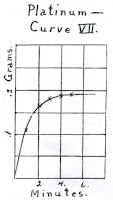
A1-Digital Scanning

Using the scanned handwritten graph found in the College of Science Library.
from

Title: Electrolytic Determinations & Separations with the Use of a Rotating Anode.

Reference: J. Langness, The Journal of the American Chemical Soc. 29, 459-472 (1907). For x-axis, the major grid is 2 and for the y-axis the major grid is 0.05.

I have found out that the pixel values for x and y are 60.75 and 58.16667 respectively. Finding the pixel locations of each point including the origin we have found the following data.

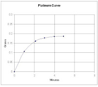
The second and third columns are the pixel locations of the data points. The fourth and fifth columns are the points when the pixel location of a data is subtracted to the pixel location of the origin. However, in the x-axis I use the absolute value.
The last two columns are the ratio of the x and y. We multiply the value of the major grid to the value of the pixel location and divide it by the pixel value. For example, data point 1(x-axis)

(2*30)/60.75 = 0.987654

Finding the ratio for all points in x and y and plotting it in excel.
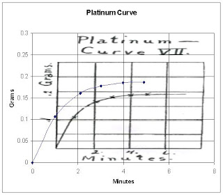
Comparing the two graphs,


I have found out that the graphs are almost the same. But because of human error of looking at the exact value of the data points, the graph will look like this.


I made some errors but I still did my best so I will give myself 10/10...

Credits to:

Elizabeth Ann Prieto for scanning the images and for answering some of my questions... :D
Good day.. :)