A4 – Enhancement by Histogram Manipulation

The task for this activity is to enhanced an image using histogram manipulation.

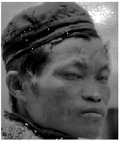
For this activity, we are asked to find grayscale images. I looked for an image in the web. The image is from: http://upload.wikimedia.org/wikipedia/commons/thumb/9/90/Face_sapa14.jpg/800px-Face_sapa14.jpg



To find the histogram of the image:

Change the directory where the image is saved.

img = imread('face.jpg');

// plot histogram
gsval=[];
pixelnum=[];
counter=1;
for i=0:1:255
[x,y]=find(img==i);
gsval(counter)=i;
pixelnum(counter)=length(x);
counter = counter+1;
end;
scf(1);
plot(gsval,pixelnum);
// puts the titles
xtitle( 'Histogram') ;

This will show


Note: x-axis is the grayscale values and the y-axis is the number of pixels.
It ii show in the histogram that the grayscale values is well spread in the image.

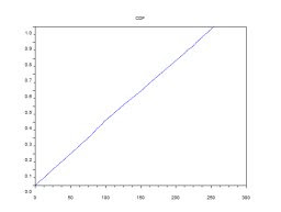
After finding the histogram, we can find the probability distribution function (PDF). PDF can be find by normalizing the pixel values of the histogram. After finding the PDF, we will find the cumulative distribution function (CDF).
To find the PDF (normalized histogram) and CDF
//plot PDF
a = gsval;
b = pixelnum;
c = size(img,1);
d = size(img,2);
e = c.*d
f = b/e;
scf(2);
plot(a,f);
g = cumsum(f);
xtitle ('Normalized Histogram')
Note: x-axis is the grayscale image and the y-axis is the normalized number of pixels.

//plot CDF
scf(3);
plot(a,g);
xtitle('CDF');

Note: x-axis is the grayscale values while y-axis is the cumulative sum of the normalized number of pixels.

________________________________________________________

Then the next thing to do is the Back Projection of the Image

//Back Projection
gray = [];
for ii = 1:1:size(img,1)
for jj = 1:1:size(img,2)
gray(ii,jj) = g(img(ii,jj));
end
end
imwrite(gray, 'gray.jpg');

After back projection,





Then we will find the histogram and the CDF of the new image.

// New Histogram
im = imread('gray.jpg');
gval=[];
pnum=[];
count=1;
for i=0:1:255
[x1,y1]=find(im==i);
gval(count)=i;
pnum(count)=length(x1);
count = count+1;
end;
scf(4);
plot(gval,pnum);
xtitle('Histogram');
Note: x-axis is the grayscale values and the y-axis is the number of pixels.

// New PDF and CDF
//plot PDF
h = gval;
i = pnum;
j = size(im,1);
k = size(im,2);
l = j.*k;
m = i/l;
plot(h,m);
xtitle('Normalized Histogram')

Note: x-axis is the grayscale image and the y-axis is the normalized number of pixels.

//plot new CDF
n= cumsum(m);
scf(5);
plot(h,n);
xtitle(' CDF');
Note: x-axis is the grayscale values while y-axis is the cumulative sum of the normalized number of pixels.

After finding the PDF and CDF of the new image. These plots show that the new image has a good contrast.

_________________________________________________________

The next task is to remap the CDF of the grayscale image to find the desired CDF.
I used the function
G = 0.5*[tanh(6*((Z-128)/255))+1] where Z = [0:255]
The graph of this function is our desired CDF
Applying the function by interpolation.

Z = [0:255];
G = tanh(6.*(Z-128)./255);
G = (G+1)/2;
A = interp1(a,g,img);
graynew = interp1(G,Z,A);

imshow(graynew, [0 255]);
The final image is
We then find the histogram, PDF and CDF using same commands we used in finding the histogram, PDF and CDF of the original image.
Histogram:
Note: x-axis is the grayscale values and the y-axis is the number of pixels.

PDF:
Note: x-axis is the grayscale image and the y-axis is the normalized number of pixels.

CDF:
Note: x-axis is the grayscale values while y-axis is the cumulative sum of the normalized number of pixels.

Comparing the three images:




The last image is darker than the other two but I think that the middle image has the best contrast. This is also based on the PDF and CDF of the images.

Acknowledgements:
Julie D.
Ed
Beth
Angel
Aiyin
for helping me and answering my questions.

Grade :
10/10, because I did my best and I enhanced the original image.